Network Analysis in Python
Laila A. Wahedi, PhD
Massive Data Institute Postdoctoral Fellow
McCourt School of Public Policy
Follow along:
- Slides: http://Wahedi.us, Tutorial
- Interactive Notebook: https://notebooks.azure.com/Laila/projects/mdi-network-analysis-workshop
Follow Along
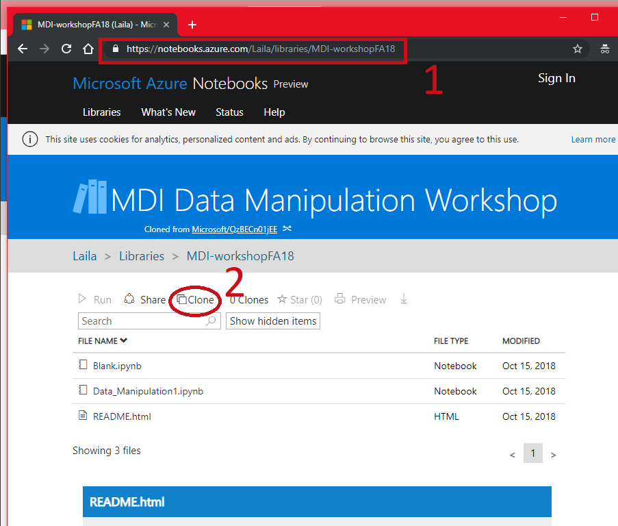
- Go to https://notebooks.azure.com/Laila/projects/mdi-network-analysis-workshop
- Clone the directory
Follow Along
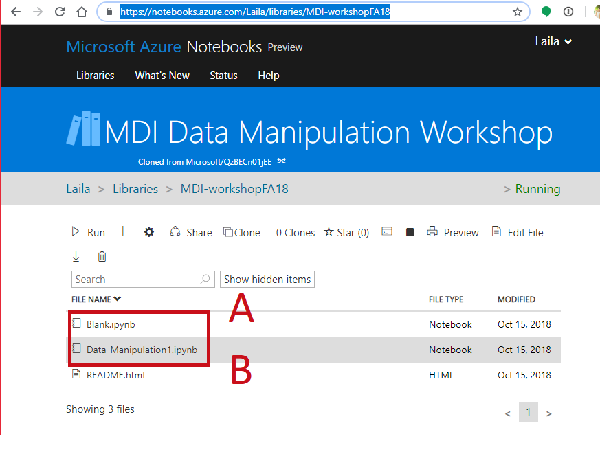
- Sign in with any Microsoft Account (Hotmail, Outlook, Azure, etc.)
- Create a folder to put it in, mark as private or public

Follow Along
- Open a notebook
- Open this notebook to have the code to play with
- Open a blank notebook to follow along and try on your own.
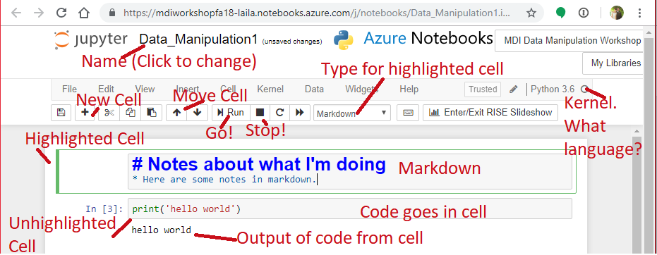
Your Environment
- Jupyter Notebook Hosted in Azure
- Want to install it at home?
- Install the Anaconda distribution of Python https://www.anaconda.com/download/
- Install Jupyter Notebooks http://jupyter.org/install
In [1]:
foo = 'some variable content'
In [2]:
print(foo)
Your Environment: Saving
- If your kernel dies, data are gone.
- Not R or Stata, you can't save your whole environment
- Data in memory more than spreadsheets
- Think carefully about what you want to save and how.
Easy Saving: Pickle
- dump to save the data to hard drive (out of memory)
Contents of the command:
- variable to save,
- File to dump the variable into:
- open(
"name of file in quotes",
"wb") "Write Binary"
- open(
Note: double and single quotes both work
In [ ]:
mydata = [1,2,3,4,5,6,7,8,9,10]
pickle.dump(mydata, open('mydata.p','wb'))
mydata = pickle.load(open("mydata.p","rb"))
Get your environment ready
- We'll cover the basics later, for now start installing and loading packages by running the following code:
In [4]:
import networkx as nx
import pandas as pd
import numpy as np
import pickle
import itertools
import matplotlib.pyplot as plt
import pysal as ps
import statsmodels.api as sm
%matplotlib inline
Before Constructing a Network...
What Do We Want From Relational Data?
Types of Analysis:
Types of Analysis:
Types of Analysis:
Types of Analysis:
Types of Analysis:
Types of Analysis:
Types of Analysis:
Types of Analysis:
Types of Analysis:
Asking Network Questions
- Hypothesize about behavior or a structural constraint
- Behavior: People make friends with those with similar interests (Homophily)
- Structural Constraint: People are more likely to interact with others close by
- How do you expect that behavior to affect the network, or vice versa
- Homophily should lead to clustering
- Expect geographic clusters of friends
- Are there other hypotheses that predict the same observed network? Can you distinguish them?
- Is clustering centered on attributes or geography? How much is due to which?
- Is the expected pattern more prevelant in the observed network than a random network?
- What is the probability that your network could have been generated randomly without your hypothesized dynamic?
- Regression: Does an individual attribute correlate with an expected pattern?
In [5]:
florentine = nx.generators.social.florentine_families_graph()
nx.draw_networkx(florentine)

In [6]:
karate = nx.generators.social.karate_club_graph()
nx.draw_networkx(karate)

Karate Club:
- A fight broke out between an administrator and instructor, breaking the club into two organizations.
- Hypothesis: Pre-existing friendships influence which side individuals will pick in a fight
- Alt-Hypothesis: People will side with the person they think is right in a conflict
- Test: Does clustering of friendships predict who will join which new karate club?
Community Detection: Review
- Divide the network into subgroups using different algorithms
- Girvan Newman Algorithm: Remove ties with highest betweenness, continue until network broken into desired number of communities
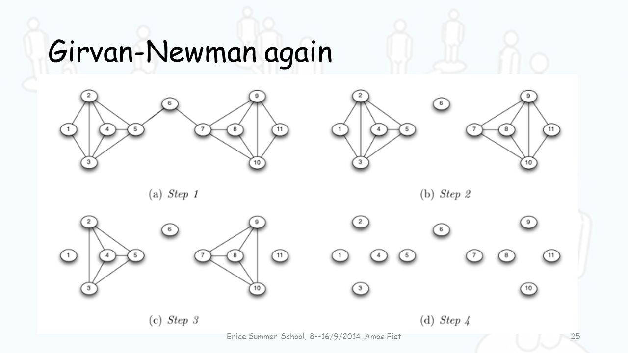
Image from: https://slideplayer.com/slide/4607021/
Community Detection: Modularity Maximization
Find divide that maximizes internal connections, minimizes external connections
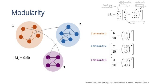 Image from https://www.slideshare.net/ErikaFilleLegara/community-detection-with-networkx-59540229
Community Detection: Modularity Maximization
- Find divide that maximizes internal connections, minimizes external connections
Image from https://www.slideshare.net/ErikaFilleLegara/community-detection-with-networkx-59540229
Modularity Maximization Algorithms
- As graphs get bigger, impossible to try all combinations of divisions to find the best one.
- Different algorithms try to maximize modularity in different ways
- leidenalg implements package one of the best, works with igraph.
- python-louvain/ community work with networkx
- Built-in Networkx algorithm for unweighted undirected networks
In [7]:
modular_communities = nx.algorithms.community.modularity_max.greedy_modularity_communities
greedy_comms = modular_communities(karate)
How did they do?
In [55]:
boundary = nx.algorithms.boundary.edge_boundary
print('quality: ',nx.algorithms.community.quality.performance(karate,greedy_comms),
     'density: ',nx.density(karate))
for i,com in enumerate(greedy_comms):
    n = len(nx.subgraph(karate,com).edges)
    b = [len(list(boundary(karate,com,c))) for c in greedy_comms[:i]+greedy_comms[i+1:]]
    d = nx.density(nx.subgraph(karate,com))
    print('internal edges: ',n, 'external edges: ',sum(b), 'density: ',d)
Okay, but we got three and there were two sides to the fight. Let's try Newman Grivan
In [8]:
ng_comms = nx.algorithms.community.centrality.girvan_newman(karate)
for com in itertools.islice(ng_comms,1):
    ng_comms = [c for c in com]
How did Newman Grivan do?
In [65]:
print('quality: ',nx.algorithms.community.quality.performance(karate,ng_comms),
     'density: ',nx.density(karate))
for i,com in enumerate(ng_comms):
    n = len(nx.subgraph(karate,com).edges)
    b = [len(list(boundary(karate,com,c))) for c in greedy_comms[:i]+ng_comms[i+1:]]
    d = nx.density(nx.subgraph(karate,com))
    print('internal edges: ',n, 'external edges: ',sum(b), 'density: ',d)
High overlap, one NG community contains two greedy communities
In [66]:
print(ng_comms)
print(greedy_comms)
In [9]:
greedy_2 = [set(greedy_comms[0]), set(greedy_comms[1]).union(greedy_comms[2])]
How is the new set?
- Slightly better, we'll use it
In [74]:
boundary = nx.algorithms.boundary.edge_boundary
print('quality: ',nx.algorithms.community.quality.performance(karate,greedy_2),
     'density: ',nx.density(karate))
for i,com in enumerate(greedy_2):
    n = len(nx.subgraph(karate,com).edges)
    b = [len(list(boundary(karate,com,c))) for c in greedy_comms[:i]+greedy_2[i+1:]]
    d = nx.density(nx.subgraph(karate,com))
    print('internal edges: ',n, 'external edges: ',sum(b), 'density: ',d)
Who Joined What Club?
- We did pretty well!
In [133]:
membership = [{0, 1, 2, 3, 4, 5, 6 , 7, 8, 10, 11, 12, 13, 16, 17, 19, 21},
              {9, 14, 15, 18, 20, 22, 23, 24, 25, 26, 27, 28, 29, 30, 31, 32, 33}]
Visualizing The Network and Results
- Matplotlib package, imported as plt
- %matplotlib inline magic to make it plot in the notebook
In [407]:
adj_labeled = nx.to_pandas_adjacency(florentine)
order = adj_labeled.sum().sort_values().index
adj_labeled = adj_labeled.loc[order,order]
plt.figure(figsize = (8,6))
plt.pcolor(adj_labeled,cmap=plt.cm.RdBu)
plt.yticks(np.arange(0.5, len(adj_labeled.index), 1), adj_labeled.index, fontsize = 20)
plt.xticks(np.arange(0.5, len(adj_labeled.index), 1), adj_labeled.columns, rotation =45, ha='right', fontsize=20 )
plt.title('Adjacency\n',fontsize=20)
cbar =plt.colorbar()

Graph Plotting Algorithms
- Can learn something by placing the nodes in an intelligent way
- Spring Algorithm: Put nodes that are connected closer together
In [145]:
plt.figure(figsize=(15,15))
pos = nx.spring_layout(karate)
deg = nx.degree(karate)
deg = [deg[k]*400 for k in karate.nodes]
nx.draw_networkx(karate,pos=pos, with_labels=True,
                node_size=deg,font_size=30)

Add Color
In [146]:
plt.figure(figsize=(15,15))
colors = []
for n in karate.nodes:
    if n in greedy_2[0]:
        colors.append('blue')
    else:
        colors.append('red')
nx.draw_networkx(karate,pos=pos, with_labels=True,
                node_size=deg,font_size=30, node_color = colors,alpha=.5)

Add Membership
In [147]:
plt.figure(figsize=(15,15))
m1 = [n for n in karate.nodes if n in membership[0]]
m1_col = [colors[i] for i, n in enumerate(karate.nodes) if n in membership[0]]
m1_deg = [deg[i] for i, n in enumerate(karate.nodes) if n in membership[0]]
m2 = [n for n in karate.nodes if n in membership[1]]
m2_col = [colors[i] for i, n in enumerate(karate.nodes) if n in membership[1]]
m2_deg = [deg[i] for i, n in enumerate(karate.nodes) if n in membership[1]]
nx.draw_networkx_nodes(nx.subgraph(karate,m1),pos=pos, alpha=.5,
                node_size=m1_deg, node_color = m1_col, node_shape='s',)
nx.draw_networkx_nodes(nx.subgraph(karate,m2),pos=pos,alpha=.5,
                node_size=m2_deg, node_color = m2_col,)
nx.draw_networkx_labels(karate, pos=pos,font_size=30,)
nx.draw_networkx_edges(karate,pos=pos,with_labels=True)
Out[147]:

In [408]:
from pysal.weights.weights import W as inst_weights
y = []
x = []
f = 0
for n in karate.nodes:
#     x.append()
    if f:
        x.append([1,0])
        f=0
    else:
        x.append([0,1])
        f =1
    if n in membership[0]:
        y.append(0)
    else: y.append(1)
x = np.array(x)
y = np.array([y]).T
neighbors = {n: list(karate[n].keys()) for n in karate.nodes}
neighbors = inst_weights(neighbors)
neighbors.transform='r'
m = ps.spreg.GM_Lag(y,x,w=neighbors, spat_diag=True,)
print(m.summary)
Hypothesize About Network Construction
- Karate Network: Network represents friendships
- Hypothesis Friends of friends are more likely to become friends
- Expectation: See more triangles than random
In [212]:
n = len(karate.nodes)
den = nx.density(karate)
t = nx.triangles(karate)
t = sum([t[i] for i in t])
triangles = []
for sim in range(500):
    g = nx.gnp_random_graph(n,den)
    tri = nx.triangles(g)
    triangles.append(sum(tri[i] for i in tri))
(t-np.mean(triangles))/np.std(triangles)
Out[212]:
Other metrics to compare
- Degree distribution
- Centrality distribution
- Centralization
Centrality Distributions
- Random graph above assumes every pair has the same probability of having an edge.
- Each node therefore has on average the same number of ties (expected degree)
- Many real networks follow a power law
- More nodes than expected have many ties or few ties
- Distribution of degree has fat tails
- Are there super popular hubs? Are there lots of loners or individuals with only one tie?
In [213]:
deg = [i[1] for i in nx.degree(karate)]
g_deg = [i[1] for i in nx.degree(g)]
pd.DataFrame({'karate':deg,'random':g_deg}).plot.hist(alpha = .5)
Out[213]:

Florentine Network
- What do you expect the degree distribution to look like?
- Why?
- Calculate it and see
In [217]:
deg = [i[1] for i in nx.degree(florentine)]
g = nx.gnp_random_graph(len(florentine.nodes),nx.density(florentine))
g_deg = [i[1] for i in nx.degree(g)]
pd.DataFrame({'karate':deg,'random':g_deg}).plot.hist(alpha = .5)
Out[217]:

Degree Distribution and Network Structure
In [268]:
g = nx.Graph()
g.add_nodes_from(list(range(16)))
g.add_edges_from([(0,1),(0,2),(0,3),(0,4),(0,5),
                 (6,7),(6,8),(6,9),(6,10),(7,8),(7,9),(7,10),(8,9),(8,10),(9,10),
                 (11,14),(11,15),(12,13),(12,16),(13,15),(14,15),(14,12)])
pos = nx.spring_layout(g,k=.65)
nx.draw_networkx(g,pos=pos)

Centralization
- How central the most central node is in relation to all others
- Centralized graphs have one or a few highly prominent nodes
- Decentralized graphs have more equal distribution of influence
- Strong implications for behavior and information flow
Sum of difference between highest centrality node and all others, divided by the max difference for network of the same size
In [264]:
def centralization(g):
    deg = [i[1] for i in nx.degree(g)]
    max_deg = max(deg)
    N = len(g.nodes)-1
    numerator = sum([max_deg -i for i in deg])
    denomenator = (N-1)**2
    return numerator/denomenator
Centralization
- Extent to which graph has some nodes that are much more prominent than others
- Centralized graphs have one or a few highly prominent nodes
- Decentralized graphs have more equal distribution of influence
- Strong implications for behavior and information flow
In [269]:
print(centralization(nx.subgraph(g,list(range(6)))))
print(centralization(nx.subgraph(g,list(range(6,11)))))
print(centralization(nx.subgraph(g,list(range(11,17)))))
nx.draw_networkx(g,pos=pos)
Proper Baselines: Random Networks Capturing These Dynamics
- Compare network to one exhibiting the traits you care about ## Preferential Attachment
- Notable individuals are easier to notice, or more desireable, and therefore gain ties faster than less well-connected nodes
- Barabasi Albert Graph: Nodes introduced sequentially, form ties to existing nodes
- set number of nodes, how many ties each forms
In [285]:
g=nx.barabasi_albert_graph(len(florentine.nodes),2)
nx.draw_networkx(g)
print(centralization(g))

Compare the preferential attachment graph to others
- Barabasi Albert graph degree distribution to Karate and Erdos Renyi
- Compare centralization to Karate and Erdos Renyi
In [290]:
g=nx.barabasi_albert_graph(len(karate.nodes),2)
g_rand = nx.erdos_renyi_graph(len(karate.nodes),nx.density(g))
print('ER centralization: ',centralization(g_rand))
print('Karate centralization: ',centralization(karate))
pd.DataFrame({'Karate': [i[1] for i in nx.degree(karate)],
             'Erdos Renyi': [i[1] for i in nx.degree(g_rand)],
             'Barabasi Albert': [i[1] for i in nx.degree(g)]}
            ).plot.hist(alpha=.5)
Out[290]:


Case Study: Senate Co-Sponsorship
- Nodes: Senators
- Links: Sponsorship of the same piece of legislation.
- Weighted
Download here:
https://dataverse.harvard.edu/file.xhtml;jsessionid=e627083a7d8f43616bbe7d4ada3e?fileId=615937&version=RELEASED&version=.0Start with the cosponsors.txt file
- Similar to an edgelist for a bipartite graph
- Each line is a bill
- Each line lists all cosponsors
Load The Cosponsor Data
- Instantiate a list for the edgelist
- Open the file
- Loop through lines
- Store the lines
In [449]:
edges = []
with open('Cosponsors.txt') as d:
    for line in d:
        edges.append(line.split())
Subset the Data: Year
2000
- Download dates.txt
- Each row is the date
- Year, month, day separated by "-"
In [450]:
dates = pd.read_csv('Dates.txt',sep='-',header=None)
dates.columns = ['year','month','day']
index_loc = np.where(dates.year==2000)
edges_00 = [edges[i] for i in index_loc[0]]
Subset the Data: Senate
- Download senate.csv
- Gives the ids for senators
- Filter down to the rows for 106th congress (2000)
This gives us our nodes
- Instantiate adjacency matrix of size nxn
- Create an ordinal index so we can index the matrix
- Add an attribute
In [451]:
# Get nodes
senate = pd.read_csv('Senate.tab',sep='\t')
senators = senate.loc[senate.congress==106,['id','party']]
# Creae adjacency matrix
adj_mat = np.zeros([len(senators),len(senators)])
senators = pd.DataFrame(senators)
senators['adj_ind']=range(len(senators))
# Create Graph Object
senateG= nx.Graph()
senateG.add_nodes_from(senators.id)
party_dict = dict(zip(senators.id,senators.party))
nx.set_node_attributes(senateG, name='party',values=party_dict)
Create the network (two ways)
- Loop through bills
- Check that there's data, and that it's a senate bill
- Create pairs for every combination of cosponsors ### Add directly to NetworkX graph object
- Add edges from the list of combinations
- Not weighted ### Add to adjacency matrix using new index
- Identify index for each pair
- Add to adjacency matrix using index
In [452]:
for bill in edges_00:
    if bill[0] == "NA": continue
    bill = [int(i) for i in bill]
    if bill[0] not in list(senators.id): continue
    combos = list(itertools.combinations(bill,2))
    senateG.add_edges_from(combos)
    for pair in combos:
        i = senators.loc[senators.id == int(pair[0]), 'adj_ind']
        j = senators.loc[senators.id == int(pair[1]), 'adj_ind']
        adj_mat[i,j]+=1
        adj_mat[j,i]+=1
Set edge weights for Network Object
In [453]:
for row in range(len(adj_mat)):
    cols = np.where(adj_mat[row,:])[0]
    i = senators.loc[senators.adj_ind==row,'id']
    i = int(i)
    for col in cols:
        j = senators.loc[senators.adj_ind==col,'id']
        j = int(j)
        senateG[i][j]['bills']=adj_mat[row,col]
Thresholding
- Some bills have everyone as a sponsor
- These popular bills are less informative, end up with complete network
- Threshold: Take edges above a certain weight (more than n cosponsorships)
- Try different numbers
In [481]:
bill_dict = nx.get_edge_attributes(senateG,'bills')
elarge=[(i,j) for (i,j) in bill_dict  if bill_dict[(i,j)] >25]
Look at the network
- Different layouts possible:
https://networkx.github.io/documentation/networkx-1.10/reference/drawing.html
In [482]:
plt.figure(figsize=(15,15))
pos = nx.spring_layout(senateG,k=.6)
deg = [(i[1]**2)/2700 for i in nx.degree(senateG, weight='bills')]
nx.draw_networkx(senateG, pos=pos, edgelist = elarge,
                 node_size = deg, with_labels=True)

Take out the singletons to get a clearer picture:
In [483]:
plt.figure(figsize=(15,15))
senateGt= nx.Graph()
senateGt.add_nodes_from(senateG.nodes)
senateGt.add_edges_from(elarge)
deg = senateGt.degree()
rem = [n[0] for n in deg if n[1]==0]
senateGt_all = senateGt.copy()
senateGt.remove_nodes_from(rem)
deg = [(i[1])**1.7 for i in nx.degree(senateGt, weight='bills')]
pos = nx.spring_layout(senateGt,k=.7)
nx.draw_networkx(senateGt,pos=pos,node_size =deg, with_labels=True)

Look at the degree distribution
In [485]:
pd.DataFrame({'weighted':[(i[1]) for i in nx.degree(senateGt, weight='bills')],
                          }).plot.hist()
Out[485]:

In [486]:
party = nx.get_node_attributes(senateG,'party')
dems = []
gop = []
for i in party:
    if party[i]==100: dems.append(i)
    else: gop.append(i)
Prepare the Visualization
- Create positional coordinates for the groups with ties, and without ties
- Instantiate dictionaries to hold different sets of coordinates
- Loop through party members
- If they have no parters, add calculated position to the lonely dictionary
- If they have partners, add calculated position to the party dictionary
In [487]:
pos = nx.spring_layout(senateGt,k=.65)
pos_all = nx.circular_layout(senateG)
dem_dict={}
gop_dict={}
dem_lone = {}
gop_lone= {}
for n in dems:
    if n in rem: dem_lone[n]=pos_all[n]
    else:dem_dict[n] = pos[n]
for n in gop:
    if n in rem: gop_lone[n]=pos_all[n]
    else:gop_dict[n] = pos[n]
Visualize the network by party
- Create lists of the party members who have ties
- Draw nodes in four categories using the position dictionaries we created
- party members, untied party members
In [488]:
plt.figure(figsize=(15,15))
dems = list(set(dems)-set(rem))
gop = list(set(gop)-set(rem))
nx.draw_networkx_nodes(senateGt, pos=dem_dict, nodelist = dems,node_color='b',node_size = 100)
nx.draw_networkx_nodes(senateGt, pos=gop_dict, nodelist = gop,node_color='r', node_size = 100)
nx.draw_networkx_nodes(senateG, pos=dem_lone, nodelist = list(dem_lone.keys()),node_color='b',node_size = 200)
nx.draw_networkx_nodes(senateG, pos=gop_lone, nodelist = list(gop_lone.keys()),node_color='r', node_size = 200)
nx.draw_networkx_edges(senateGt,pos=pos, edgelist=elarge)
Out[488]:

Do it again with a higher threshold:
In [490]:
elarge=[(i,j) for (i,j) in bill_dict  if bill_dict[(i,j)] >35]
plt.figure(figsize=(15,15))
dems = list(set(dems)-set(rem))
gop = list(set(gop)-set(rem))
nx.draw_networkx_nodes(senateGt, pos=dem_dict, nodelist = dems,node_color='b',node_size = 100)
nx.draw_networkx_nodes(senateGt, pos=gop_dict, nodelist = gop,node_color='r', node_size = 100)
nx.draw_networkx_nodes(senateGt_all, pos=dem_lone, nodelist = list(dem_lone.keys()),node_color='b',node_size = 100)
nx.draw_networkx_nodes(senateGt_all, pos=gop_lone, nodelist = list(gop_lone.keys()),node_color='r', node_size = 100)
nx.draw_networkx_edges(senateGt,pos=pos, edgelist=elarge)
Out[490]:

Hypothesis: Homophily
- Excpect senators who have more similar beliefs (in same party) to co-sponsor bills more often
- Use the greedy algorithm to generate communities
In [462]:
colors = modular_communities(senateGt, weight = 'bills')
Visualize the Communities
- Calculate a position for all nodes
- Separate network by the communities
- Draw the first set as red
- Draw the second set as blue
- Add the edges
In [463]:
elarge=[(i,j) for (i,j) in bill_dict  if bill_dict[(i,j)] >35]
plt.figure(figsize=(15,15))
pos = nx.spring_layout(senateGt)
pos0={}
pos1={}
for n in colors[0]:
    pos0[n] = pos[n]
for n in colors[1]:
    pos1[n] = pos[n]
nx.draw_networkx_nodes(senateGt, pos=pos0, nodelist = colors[0],node_color='r')
nx.draw_networkx_nodes(senateGt, pos=pos1, nodelist = colors[1],node_color='b')
nx.draw_networkx_edges(senateGt,pos=pos, edgelist=elarge)
Out[463]:

In [465]:
print('gop misclassification')
for i in colors[0]:
    if i in dems: print(i,len(senateGt[i]))
print('dem misclassification')
for i in colors[1]:
    if i in gop: print(i,len(senateGt[i]))
Pretty, but now what?
Structure is interesting itself
- Is polarization changing over time?
- What attributes of a senator or environment lead to more in-party cosponsorship.
- Use ERGM or Latent Space Model
- Beyond what we'll cover today, but check out:
- Edward's implementation of Latent Space Models: http://edwardlib.org/tutorials/latent-space-models
- Statnet's ERGM implementation in R: https://statnet.org/trac/raw-attachment/wiki/Sunbelt2016/ergm_tutorial.html
Research Questions
Effects of networks
- How does a congressman's betweenness centrality affect their committee placement?
- How does a congressman's degree centrality affect their reelection?
- How does a party's modularity affect their ability to accomplish their agenda
- Does the behavior of tied nodes affect the behavior of a node?
- Is there diffusion across the network?
Use Network Variables in Your Regression
- Control for centrality measures or other positional effects
- Party or community as unit of analysis
- Use network lags to account for interdependence (adapt a var or spatial lag model)
- Remember, if you use spatial lags, you need to correct for it in your error term to get unbiased standard errors
- p(y) conditional on y for neighboring nodes
- Learn more here. Use your adjacency matrix for W instead of distance decay function. http://www.statsref.com/HTML/index.html?car_models.html
Load some more data from Fowler
- SH file
- .tab or .csv, depending on source
- pb: sponsored bills passing chamber
- pa: sponsored ammendments passing chamber
In [466]:
sh = pd.read_csv('SH.tab',sep='\t')
sh['dem']= sh.party==100
sh['dem']=sh.dem*1
model_data = sh.loc[
    (sh.congress == 106) & (sh.chamber=='S'),
    ['ids','dem','pb','pa']
]
model_data['passed']=model_data.pb+model_data.pa
model_data.set_index('ids',inplace=True)
Merge in some network data
- Remember: The merge works because they have the same index
In [467]:
deg_cent = nx.degree_centrality(senateGt)
deg_cent = pd.Series(deg_cent)
model_data['degree']=deg_cent
Degree is not significant
In [468]:
y =model_data.loc[:,'passed']
x =model_data.loc[:,['degree','dem']]
x['c'] = 1
ols_model1 = sm.GLM(y,x,missing='drop',family=sm.families.NegativeBinomial())
results = ols_model1.fit()
print(results.summary())
What about Betweenness?
In [ ]:
bet_cent = nx.closeness_centrality(senateG,weight='bills',)
bet_cent = pd.Series(bet_cent)
model_data['between']=bet_cent
y =model_data.loc[:,'passed']
x =model_data.loc[:,['between','dem']]
x['c'] = 1
model1 = sm.GLM(y,x,missing='drop',family=sm.families.NegativeBinomial())
results = model1.fit()
print(results.summary())