Network Analysis in Python
Laila A. Wahedi, PhD
Massive Data Institute Postdoctoral Fellow
McCourt School of Public Policy
Follow along:
- Slides: http://Wahedi.us, Tutorial
- Interactive Notebook: https://notebooks.azure.com/Laila/projects/mdi-network-analysis-workshop
Follow Along
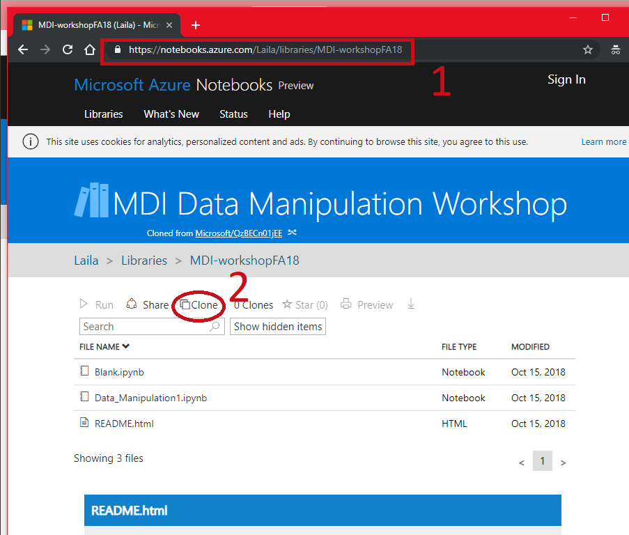
- Go to https://notebooks.azure.com/Laila/libraries/MDI-workshopFA18
- Clone the directory
Follow Along
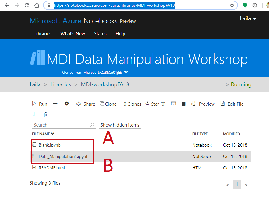
- Sign in with any Microsoft Account (Hotmail, Outlook, Azure, etc.)
- Create a folder to put it in, mark as private or public

Follow Along
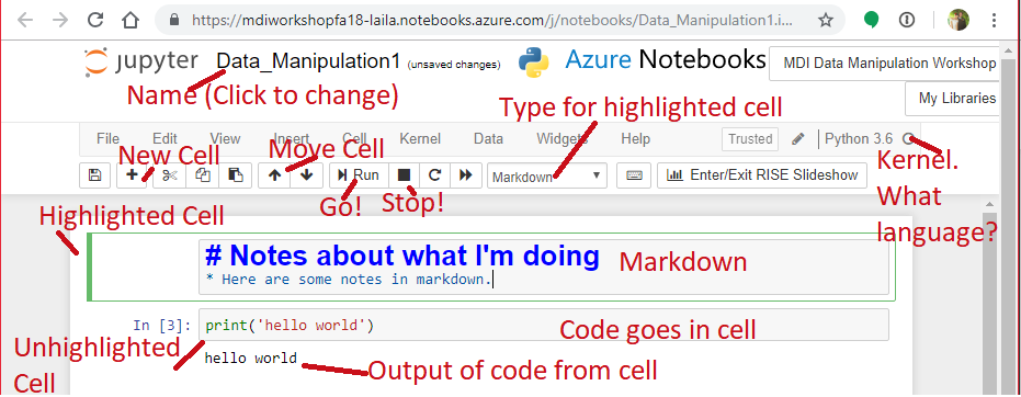
- Open a notebook
- Open this notebook to have the code to play with
- Open a blank notebook to follow along and try on your own.
Your Environment
- Jupyter Notebook Hosted in Azure
- Want to install it at home?
- Install the Anaconda distribution of Python https://www.anaconda.com/download/
- Install Jupyter Notebooks http://jupyter.org/install
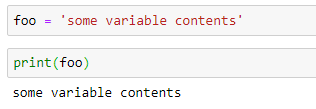
In [1]:
foo = 'some variable content'
In [2]:
print(foo)
Your Environment: Saving
- If your kernel dies, data are gone.
- Not R or Stata, you can't save your whole environment
- Data in memory more than spreadsheets
- Think carefully about what you want to save and how.
Easy Saving: Pickle
- dump to save the data to hard drive (out of memory)
Contents of the command:
- variable to save,
- File to dump the variable into:
- open(
"name of file in quotes",
"wb") "Write Binary"
- open(
Note: double and single quotes both work
In [ ]:
mydata = [1,2,3,4,5,6,7,8,9,10]
pickle.dump(mydata, open('mydata.p','wb'))
mydata = pickle.load(open("mydata.p","rb"))
Get your environment ready
- We'll cover the basics later, for now start installing and loading packages by running the following code:
In [2]:
import networkx as nx
import pandas as pd
import numpy as np
import pickle
import matplotlib.pyplot as plt
%matplotlib inline
What is a network?
- Nodes/ Vertices
- Links/ edges/ ties/ arcs
- Weights
- Also called a graph
Bipartite: Networks with two types of node
- People and the stores they shop in
- Movies and actors
- Words and authors
- What are some other examples?
Weighted: Networks with ties of different strength
- Twitter users linked by number of retweets
- People linked by distance between homes
- Cities linked by dollars of trade
- Cities linked by number of travelers
Directed Networks:
Edges are not always symmetrical
- Twitter user @Ahmad may retweet @Bethany more often than @Bethany retweets Ahmad
- Mexico buys from the US more than the US buys from Mexico
- User mentions on Twitter
- Outgoing phone calls between people
- Friendship rankings: Bobathy may list Amira as a friend on a survey without Amira listing Bobathy
Weighted and directed networks are related. Which are weighted and which are unweighted?
When are weighted networks not directed?
Representing a Network: Edge List
- Dyads
- Each row contains a pair of nodes indicating a tie
- A Third Column Cindicates weight
- Order may indicate direction of edge
In [30]:
edges = [('Fred', 'Maria'),
         ('Fred', 'Samir'),
         ('Fred', 'Jose',),
         ('Maria', 'Sonya',),
         ('Samir','Jose'),
         ('Samir','Sonya'),]
Make this a weighted, undirected network
In [25]:
edges_weighted = [('Fred', 'Maria', 3),
                 ('Fred', 'Samir', 6),
                 ('Fred', 'Jose', 2),
                 ('Maria', 'Sonya', 1),
                 ('Samir','Jose',3),
                 ('Samir','Sonya',5)]
What would you need to do to make this directed?
In [63]:
edges_directed = [('Fred', 'Maria', 3),
                 ('Fred', 'Samir', 6),
                 ('Fred', 'Jose', 2),
                 ('Maria', 'Sonya', 1),
                 ('Samir','Jose',3),
                 ('Samir','Sonya',5),
                ('Maria', 'Fred', 2),
                 ('Samir', 'Fred', 4),
                 ('Jose', 'Fred', 6),
                 ('Sonya', 'Maria', 3),
                 ('Jose','Samir',3),]
Representing a network: Adjacency Matrix
- nxn matrix of nodes, where position i,j indicates relationship between node i and node j
- Index position corresponds with nodes. Keep the order straight
- Can be symmetrical or directed, use weights or indicators with 1
- Less space efficient for sparse networks, but convenient for linear algebra operations
- Use Numpy package, imported as np to make matrices
- Index as (row, column)
- Why: Do matrix operations on whole network
Representing a network: Adjacency Matrix
In [48]:
adj = np.zeros((5,5))
edge_index = [(0,1),(0,2),(0,3),
     (1,0),(1,4),
     (2,0),(2,3),(2,4),
     (3,0),(3,2),
     (4,1),(4,2)]
for p in edge_index:
    adj[p] = 1
adj
Out[48]:
Representing a network: Adjacency Matrix
- To keep your labels, use the Pandas package, imported as pd
In [16]:
nodes = ['Fred','Maria','Samir','Jose','Sonya','Freya','Hasan']
adj_labeled = pd.DataFrame(adj,columns=nodes,index=nodes)
adj_labeled
Out[16]:
Representing A network in Python: Networkx Object
- Using the networkx package, imported as nx
- Package designed to hold network data, visualize it, and to perform basic exploratory analysis
Instantiating Our Network
- Declare a graph object
- Graph is another term for network
- Add your nodes or vertices
- Add your edges from an edgelist
In [149]:
G = nx.Graph()
G.add_nodes_from(nodes)
G.add_edges_from(edges)
G
Out[149]:
In [33]:
print(G.nodes)
In [39]:
G.edges()
Out[39]:
In [40]:
print(G['Fred'])
Add Some Friends
In [49]:
G.add_nodes_from(['Freya','Hasan'])
G.add_edges_from([('Sonya','Freya'),('Sonya','Hasan')])
In [51]:
nx.draw_networkx(G, with_labels = True)

Make a Weighted Network:
- Add weighted edges instead of unweighted edges
- Stores weight attribute in the edges
- Can also store node attributes
In [59]:
G_weighted = nx.Graph()
G_weighted.add_nodes_from(nodes)
G_weighted.add_weighted_edges_from(edges_weighted)
nx.set_node_attributes(G_weighted,
                       {'Fred':16,
                       'Maria:':15,
                       'Samir':15,
                       'Jose':15,
                       'Sonya':14},
                      'age')
Make a Directed Network:
- Use a DiGraph object
- Can also use weighted edges
- Stores weight attribute in the edges
In [79]:
G_dir = nx.DiGraph()
G_dir.add_nodes_from(nodes)
G_dir.add_weighted_edges_from(edges_directed)
nx.set_node_attributes(G_dir,
                       {'Fred':16, 'Maria:':15,
                       'Samir':15,'Jose':15,
                       'Sonya':14}, 'age')
View Your Data:
- Friends are no longer symmetrical
In [66]:
print(G_dir['Samir'])
print(G_dir['Jose'])
View Your Data:
- View node attributes
- View weights
In [81]:
G_dir.nodes['Samir']['age']
Out[81]:
In [84]:
G_dir['Samir']['Fred']['weight']
Out[84]:
Make a Bipartite Network:
- Two node sets
- Edges between node sets
- No edges within node sets
In [106]:
G_bi = nx.Graph()
G_bi.add_nodes_from(['Georgetown',
                     'George Mason',
                     'George Washington'],
                   bipartite = 0)
G_bi.add_nodes_from(['Fred','Jose',
                    'Ayesha','Sara',
                    'Bethany','Bobathy'],
                    bipartite = 1
                   )
Make a Bipartite Network:
- Two node sets
- Edges between node sets
- No edges within node sets
In [107]:
G_bi.add_edges_from([('Georgetown','Fred'),
                    ('Georgetown','Jose'),
                     ('Georgetown','Ayesha'),
                     ('George Washington','Fred'),
                    ('George Washington','Jose'),
                    ('George Washington','Sara'),
                     ('George Mason','Bethany'),
                     ('George Mason','Bobathy')
                    ])
Project to unipartite
- Ties between universities that admitted the same students
- Bipartite set treated as attribute label
In [112]:
schools = []
for node, data in G_bi.nodes(data=True):
    if data['bipartite']==0:
        schools.append(node)
G_schools = nx.bipartite.projected_graph(G_bi, schools)
nx.draw_networkx(G_schools, with_labels=True)

Make G_bi a weighted graph
In [113]:
G_bi.add_weighted_edges_from([('Georgetown','Fred',10000),
                        ('Georgetown','Jose',0),
                         ('Georgetown','Ayesha',20000),
                         ('George Washington','Fred',7000),
                        ('George Washington','Jose',10000),
                        ('George Washington','Sara',0),
                         ('George Mason','Bethany',30000),
                         ('George Mason','Bobathy',0)
                        ])
Back to the Friendship Network
- Who is most popular?
- Who is most powerful?
- Why?
In [114]:
nx.draw_networkx(G)

Degree Centrality
- Number of ties, or normalized number of ties
- Sum of rows
- In-degree: number of edges to a node
- Out-degree: number of edges from a node
- When?
In [115]:
deg = nx.degree_centrality(G)
print(deg)
Eigenvector Centrality
- Connectedness to other well-connected nodes
Theoretical Implication: A lot of work to maintain ties to everyone, sometimes just as good to know someone who knows everyone.
- Finding a job
- Rumors
- Supply
Requires connected network
- Cannot compare across networks
When might eigenvector centrality be less useful?
Calculating Eigenvector Centrality
- Take eigenvector for maximum eigenvalue
- nx.eigenvector_centrality uses a different method that usually converges to the same result, but sometimes errors.
In [116]:
eig_c = nx.eigenvector_centrality_numpy(G)
toy_adj = nx.adjacency_matrix(G)
print(eig_c)
val,vec = np.linalg.eig(toy_adj.toarray())
print(val)
vec[:,0]
Out[116]:
Betweenness Centrality
- Proportional to the number of shortest paths that pass through a given node
- How important is that node in connecting other nodes
In [117]:
betw = nx.betweenness_centrality(G)
print(betw)
Centrality Measures Are Different
- Select based on theory you want to capture
- Correlation between measures differs across networks
- Take a minute to play around with the network and see how the relationships change
In [119]:
cent_scores = pd.DataFrame({'deg':deg,'eig_c':eig_c,'betw':betw})
print(cent_scores.corr())
cent_scores
Out[119]:
Difference in Measures
- Sonya has the most friends
- Sonya's friends are not as well connected, lowering her eigenvector centrality
- Fred and Samir have better connected friends
- Hasan and Freya have no connection to the others except through Sonya, giving her high betweenness
In [120]:
nx.draw_networkx(G)

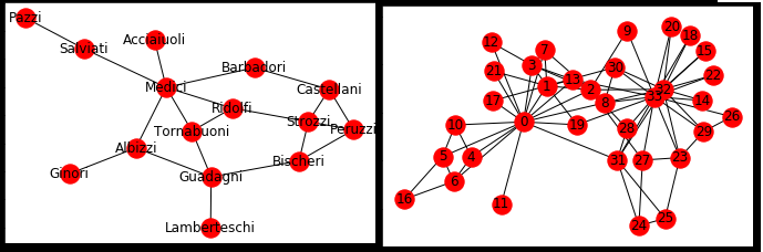
Florentine Marriage Networks
- Families in this graph are connected when there are marriage ties between them
- Calculate the centrality scores
- Who is the most powerful?
In [137]:
florentine = nx.generators.social.florentine_families_graph()
nx.draw_networkx(florentine)

Florentine Centrality
In [136]:
deg = nx.degree_centrality(florentine)
betw = nx.betweenness_centrality(florentine)
eigc = nx.eigenvector_centrality(florentine)
cent_scores = pd.DataFrame({'deg':deg,'eig_c':eigc,'betw':betw})
cent_scores.sort_values(['deg','eig_c','betw'])
Out[136]:
Florentine Centrality
- Which measure best captures Medici power? Why?
- What's up with Guadagni's betweenness vs Stozzi?
- Why does Strozzi have high eigenvector centrality?
Karate Club Graph
- Compare 0 and 32/33
- Shared influence
- Compare 5/6 with 27/28
- Neighborhood density
- Why is eigenvector better correlated with degree here than in our friend graph?
- Triangles!
In [132]:
karate = nx.generators.social.karate_club_graph()
nx.draw_networkx(karate)

Karate Club Graph
- Compare 0 and 32/33
- Shared influence
- Compare 5/6 with 27/28
- Neighborhood density
- Why is eigenvector better correlated with degree here than in our friend graph?
- Triangles!
In [139]:
deg = nx.degree_centrality(karate)
betw = nx.betweenness_centrality(karate)
eigc = nx.eigenvector_centrality(karate)
cent_scores = pd.DataFrame({'deg':deg,'eig_c':eigc,'betw':betw})
cent_scores.sort_values(['deg','eig_c','betw'])
Out[139]:
Speaking of triangles: Transitivity
- Extent to which friends have friends in common
- Probability two nodes are tied given that they have a partner in common
- Make a more transitive network:
In [146]:
G_trans = G.copy()
G_trans.add_edges_from([('Samir','Maria')])
nx.draw_networkx(G_trans)

Transitivity
- Extent to which friends have friends in common
- Probability two nodes are tied given that they have a partner in common ### Look at transitivity and triangles in the two networks
In [150]:
print("Transitivity:")
print(nx.transitivity(G))
print(nx.transitivity(G_trans))
print("Triangles:")
print(nx.triangles(G))
print(nx.triangles(G_trans))
Clustering Coefficient
- Individual Nodes:
- Proportion of possible triangles through a given node
- Whole Network
- Average clustering across whole network
In [151]:
print("Clustering coefficient")
print(nx.clustering(G))
print(nx.clustering(G_trans))
print("Average Clustering")
print(nx.average_clustering(G))
print(nx.average_clustering(G_trans))
Which is more clustered? Florentine or Karate?
Florentine has few triangles
In [158]:
nx.draw_networkx(florentine)
nx.average_clustering(florentine)
Out[158]:

Karate Club has a lot of triangles
- Why might they be different?
In [159]:
nx.draw_networkx(karate)
nx.average_clustering(karate)
Out[159]:

Different Structures Are Produced by and Produce Different Behaviors
- Triadic closure -> transitivity on friendship network
- Less redundancy in strategic Medicci marriage contracts. Triangles inefficient
- Clustering captures tendency toward closure globally. What might it miss?
What might we miss?
In [174]:
squares = nx.Graph()
se = [(0,1),(1,2),(2,3),(3,0),(0,5),(4,5),(3,4),
    (5,6),(6,7),(7,0),(2,8),(8,9)]
se2 = [(i[0]+9,i[1]+9) for i in se[:-2]]
se.extend(se2)
squares.add_nodes_from(range(17))
squares.add_edges_from(se)
nx.draw_networkx(squares)
nx.average_clustering(squares)
Out[174]:

What Can We Do?
- Count n-cycles.
- Count all cycles, keep those below threshold
In [175]:
nx.cycle_basis(squares)
Out[175]:
What Can We Do?
- Square clustering ### Intuitive names like clustering are nice, but always know what you're measuring and check if it's appropriate for your network
In [190]:
clustering_coefs = nx.square_clustering(squares).values()
np.mean(list(clustering_coefs))
Out[190]:
Community Detection
- Divide the network into subgroups using different algorithms
- Examples
- Percolation: find communities with fully connected cores
- Minimum cuts (nodes): Find the minimum number of nodes that, if removed, break the network into multiple components. Progressively remove them.
- Girvan Newman Algorithm: Remove ties with highest betweenness, continue until network broken into desired number of communities
In [145]:
coms = nx.algorithms.community.centrality.girvan_newman(G)
i = 2
for com in itertools.islice(coms,4):
    print(i, ' communities')
    i+=1
    print(tuple(c for c in com))
Why Detect Communities
- Learn something about how an unknown network is organized
- Generate hypotheses.
- Why did these communities emerge?
- How do these communities affect the behavior of members?
- How do they relate to attributes of the members?
- How do they evolve over time, how do different networks compare?
What are some examples?
Assessing Community Detection:
- Density: Number of ties / maximum number
- Maximum number of ties: Every node in network has a tie
- Modularity: Fraction of edges within a group / expected edges in random graph
- Is the density within each community greater than a random network generated with the same density of the overall network
In [198]:
nx.density(G)
Out[198]:
Preview: Random Graphs
- Different methods to capture different properties
- Compare random graph with desired properties to real graph
- Today: Erdos-Renyi Graph
- Takes all possible edges
- Each edge has a probability p of being realized
- Produces graph with desired average density
- Does not capture other properties common in real world graphs #### More next week!
In [209]:
G_rand = nx.gnp_random_graph(len(karate.nodes),
                             nx.density(karate))
nx.draw_networkx(G_rand)

Modularity and Random Graphs
- Compare number of ties within community to expected number if the graph were an Erdos Renyi Graph
In [220]:
nx.average_clustering(karate)
Out[220]:
In [221]:
nx.average_clustering(G_rand)
Out[221]:
Compare the clustering visually:
In [231]:
#View clusters
plt.hist(nx.clustering(karate).values(), alpha = .5)
plt.hist(nx.clustering(G_rand).values(), alpha = .5)
Out[231]:

Compare the clustering in florentine to a random network
- How do they differ?
In [227]:
G_rand_f = nx.gnp_random_graph(len(florentine.nodes),
                             nx.density(florentine))
nx.draw_networkx(G_rand_f)

Compare the clustering in florentine to a random network
- How do they differ?
In [230]:
print('Florentine: ',nx.average_clustering(florentine))
print('Random: ', nx.average_clustering(G_rand_f))
plt.hist(nx.clustering(florentine).values(),alpha=.5)
plt.hist(nx.clustering(G_rand_f).values(), alpha = .5)
Out[230]:

Modularity Based Performance Measurement
- Modularity: Fraction of edges within group - expected number of edges
- Networkx performance metric:
- (Number of edges within groups - Number of edges between groups)/(Total Edges)
In [318]:
coms = nx.algorithms.community.centrality.girvan_newman(squares)
for com in itertools.islice(coms,1):
    partition = tuple(list(c) for c in com)
nx.algorithms.community.quality.performance(squares,partition)
Out[318]:
Compare the insularity of the communities in the florentine and karate networks
- Why is it that so?
In [310]:
coms = nx.algorithms.community.centrality.girvan_newman(karate)
for com in itertools.islice(coms,1):
    k_partition = tuple(list(c) for c in com)
nx.algorithms.community.quality.performance(karate,k_partition)
Out[310]:
In [347]:
coms = nx.algorithms.community.centrality.girvan_newman(florentine)
for com in itertools.islice(coms,1):
    fl_partition = tuple(list(c) for c in com)
nx.algorithms.community.quality.performance(florentine,fl_partition)
Out[347]:
Visualizing the networks
- Matplotlib package, imported as plt
- %matplotlib inline magic to make it plot in the notebook
In [357]:
order = adj_labeled.sum().sort_values().index
adj_labeled = adj_labeled.loc[order,order]
plt.figure(figsize = (8,6))
plt.pcolor(adj_labeled,cmap=plt.cm.RdBu)
plt.yticks(np.arange(0.5, 5, 1), adj_labeled.index, fontsize = 20)
plt.xticks(np.arange(0.5, 5, 1), adj_labeled.columns, rotation =45, ha='right', fontsize=20 )
plt.title('Adjacency\n',fontsize=20)
cbar =plt.colorbar()

Graph Plotting Algorithms
- Can learn something by placing the nodes in an intelligent way
- Force Algorithm: Put nodes that are connected closer together
In [358]:
plt.figure(figsize=(15,15))
pos = nx.spring_layout(florentine)
deg = nx.degree(florentine)
deg = [deg[k]*400 for k in florentine.nodes]
nx.draw_networkx(florentine,pos=pos, with_labels=True,
                node_size=deg,font_size=30)

Add Color
In [359]:
plt.figure(figsize=(15,15))
colors = []
for n in florentine.nodes:
    if n in fl_partition[0]:
        colors.append('blue')
    else:
        colors.append('red')
nx.draw_networkx(florentine,pos=pos, with_labels=True,
                node_size=deg,font_size=30, node_color = colors)

Draw the Florentine Network with Three Partitions
In [360]:
coms = nx.algorithms.community.centrality.girvan_newman(florentine)
for com in itertools.islice(coms,2):
    fl_partition = tuple(list(c) for c in com)
nx.algorithms.community.quality.performance(florentine,fl_partition)
colors = []
for n in florentine.nodes:
    if n in fl_partition[0]:
        colors.append('blue')
    elif n in fl_partition[1]:
        colors.append('red')
    else:
        colors.append('green')
plt.figure(figsize=(15,15))
nx.draw_networkx(florentine,pos=pos, with_labels=True,
                node_size=deg,font_size=30, node_color = colors)

Next Time: Making Inferences
- Network Questions
- Network Properties
- Degree distributions
- Centralization
- Random Networks
- Regressions with Network Variables